T Test Calculator

This t test calculator computes t-scores, p-values, degrees of freedom, and critical values using raw data arrays or summary statistics like sample mean, standard deviation, and sample size. It eliminates guesswork when testing sample hypotheses, helping you confirm whether differences between group averages reflect real effects rather than random sampling noise. Whether you run split-testing experiments on a website or evaluate clinical lab trials, it reveals whether your experimental results reach genuine statistical significance.

One sample

H_0: \mu = \mu_0 \quad H_1: \mu \neq \mu_0

Enter data as

Sample mean *

Sample standard deviation *

Sample size *

Hypothesised mean *

Alternative hypothesis

Significance level *

Test result

Significant

One sample t test

Test statistic

t = 2.6245df = 29

p = 0.013700

p is at or below 0.05, so reject the null hypothesis.

p value in every tail

Two tailedselected

0.013700

Left tailed

0.993150

Right tailed

0.006850

Only the selected tail decides the verdict. Choose the direction before seeing the data, because picking a one tailed test afterwards roughly doubles the false positive rate.

Where the statistic falls

p value

0.013700

two tailed

Critical value

±2.0452

at alpha 0.05

Degrees of freedom

exact

Standard error

0.87636

of the estimate

95% confidence interval

50.5077 to 54.0923

for the population mean

Cohen's d

0.4792

Small effect

Hedges' g

0.4667

d corrected for small samples

Achieved power

71.7%

below the usual 80% target, approximate

Descriptive statistics

Group	n	Mean	SD
Sample	30	52.3	4.8

Assumption checks

Sample size: n = 30, the mean is safely normal by the central limit theorem

Independent observations: Each value must come from a separate unit

Created by Natasha Okonkwo

Last updated: September 26, 2026

What This T Test Calculator Does

A t-test evaluates whether the average difference between sample groups or against a known baseline is real or just luck. If you test two website layouts, measure patient recovery across drug doses, or check machine parts against factory standards, random sampling causes small variations every time.

This tool automates three distinct calculations:

Independent Two-Sample T-Test (Unpaired): Compares the means of two unrelated groups (for example, Group A vs. Group B). It supports both Student's t-test (equal variances) and Welch's t-test (unequal variances).
Paired Samples T-Test (Dependent): Compares the same subjects measured twice (such as before and after an intervention).
One-Sample T-Test: Compares a single sample mean against a known target or population standard.

The one-sample and two-sample tabs take your data in two ways: paste comma-separated raw numbers, or enter pre-calculated summary metrics (mean, standard deviation, and count). The paired tab needs the raw pairs, because a paired test depends on how each individual pair moved rather than on the two group means, so summary statistics cannot describe it. The tool outputs your test statistic ( $t$ ), degrees of freedom ( $df$ ), standard error, the $p$ -value in all three tails at once, effect size as both Cohen's $d$ and the small-sample-corrected Hedges' $g$ , the achieved power, and a confidence interval at whatever level your significance threshold implies (95% at the default $\alpha = 0.05$ , 99% at 0.01, and so on).

Choosing the Right Type of T-Test

Using the wrong test type yields inaccurate p-values and false conclusions. Select your test based on your experimental design:

Test Type	When to Choose	Practical Example
Independent (Equal Variances / Student's)	Two separate, unrelated groups with similar spreads.	Test score comparisons between Class 1 and Class 2.
Welch's T-Test (Unequal Variances)	Two separate groups where standard deviations or sample sizes differ.	Comparing revenue per user between desktop and mobile visitors.
Paired T-Test	The same subjects tested across two conditions or time periods.	Patient blood pressure before medication vs. after medication.
One-Sample T-Test	One group compared against a known fixed benchmark.	Verifying if a batch of 12-ounce soda cans actually averages 12.0 ounces.

When comparing two independent groups, Welch's t-test is generally safer than Student's classic test. It protects against unequal variances without losing statistical power when variances happen to match. If your study examines proportions rather than numerical averages, use our z test calculator instead.

T-Test Formulas and Mathematical Logic

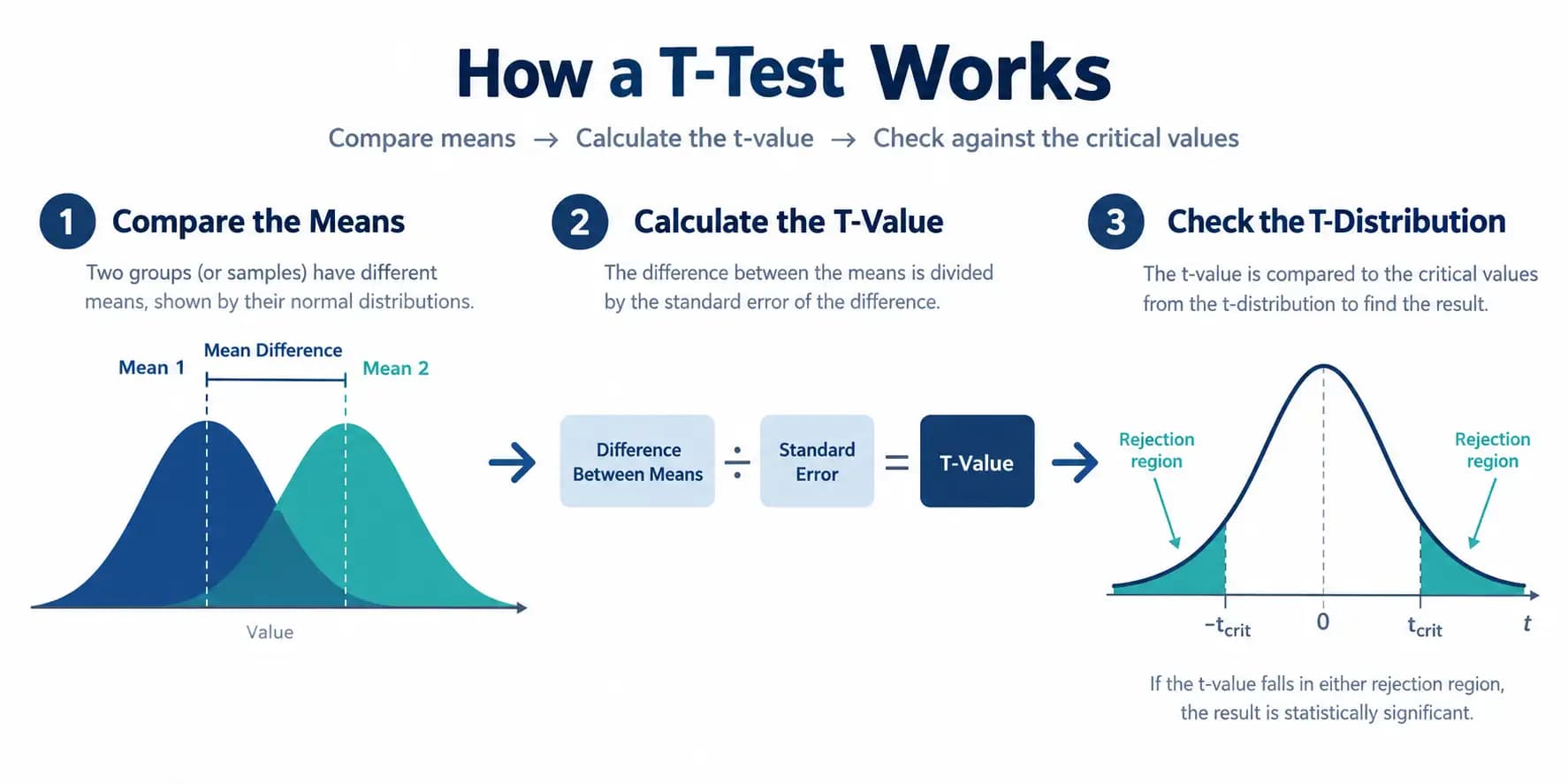
Infographic diagram showing mean differences divided by standard error to calculate t-score and p-value tails.

Every t-test divides the observed difference by the standard error of that difference. The standard error measures how much sample averages naturally bounce around due to chance.

1. One-Sample T-Test Formula

The one-sample test checks if sample mean $\bar{x}$ differs from population mean $\mu_0$ :

t = \frac{\bar{x} - \mu_0}{\frac{s}{\sqrt{n}}}

Where:

$\bar{x}$ = Sample mean
$\mu_0$ = Hypothesized population mean
$s$ = Sample standard deviation
$n$ = Sample size

Degrees of freedom: $df = n - 1$

2. Paired Samples T-Test Formula

A paired test calculates differences ( $d_i = x_{1i} - x_{2i}$ ) for each subject, then runs a one-sample test on those difference scores:

t = \frac{\bar{d} - 0}{\frac{s_d}{\sqrt{n}}}

Where:

$\bar{d}$ = Average of the individual difference scores
$s_d$ = Standard deviation of the difference scores
$n$ = Number of paired observations

Degrees of freedom: $df = n - 1$

3. Independent Two-Sample T-Test (Student's Pooled Variance)

When group variances are assumed equal ( $\sigma_1^2 = \sigma_2^2$ ), we pool standard deviations:

s_p^2 = \frac{(n_1 - 1)s_1^2 + (n_2 - 1)s_2^2}{n_1 + n_2 - 2}

t = \frac{\bar{x}_1 - \bar{x}_2}{\sqrt{s_p^2 \left(\frac{1}{n_1} + \frac{1}{n_2}\right)}}

Degrees of freedom: $df = n_1 + n_2 - 2$

4. Welch's T-Test (Unequal Variances)

When group variances differ, pooling variance introduces systematic error. Welch's t-test calculates standard error separately for each group:

t = \frac{\bar{x}_1 - \bar{x}_2}{\sqrt{\frac{s_1^2}{n_1} + \frac{s_2^2}{n_2}}}

Degrees of freedom follow the Welch-Satterthwaite equation, which often yields fractional values:

df = \frac{\left(\frac{s_1^2}{n_1} + \frac{s_2^2}{n_2}\right)^2}{\frac{\left(\frac{s_1^2}{n_1}\right)^2}{n_1 - 1} + \frac{\left(\frac{s_2^2}{n_2}\right)^2}{n_2 - 1}}

Worked Example: Comparing Two Website Landing Pages

Let us walk through a practical A/B testing scenario using summary statistics.

An e-commerce manager wants to know if redesigning a checkout page increases average order value (AOV).

Page A (Original): $n_1 = 30$ , $\bar{x}_1 = \$52.40$ , $s_1 = \$8.20$
Page B (New Design): $n_2 = 30$ , $\bar{x}_2 = \$57.10$ , $s_2 = \$9.50$
Significance level ( $\alpha$ ): 0.05 (two-tailed)

Step 1: Calculate the Mean Difference

\bar{x}_1 - \bar{x}_2 = 52.40 - 57.10 = -4.70

The new page generated $\$4.70$ higher average order value.

Step 2: Calculate Standard Errors for Each Group

\frac{s_1^2}{n_1} = \frac{(8.20)^2}{30} = \frac{67.24}{30} \approx 2.2413

\frac{s_2^2}{n_2} = \frac{(9.50)^2}{30} = \frac{90.25}{30} \approx 3.0083

Combined Standard Error ( $SE$ ):

SE = \sqrt{2.2413 + 3.0083} = \sqrt{5.2496} \approx 2.2912

Step 3: Compute the T-Score

t = \frac{-4.70}{2.2912} \approx -2.051

Step 4: Calculate Welch's Degrees of Freedom

df = \frac{(5.2496)^2}{\frac{(2.2413)^2}{29} + \frac{(3.0083)^2}{29}} = \frac{27.5583}{\frac{5.0234}{29} + \frac{9.0499}{29}} = \frac{27.5583}{0.1732 + 0.3121} = \frac{27.5583}{0.4853} \approx 56.78

Step 5: Determine P-Value and Significance

Looking up $t = -2.051$ with $df = 56.78$ in a Student's t-distribution produces:

Two-tailed p-value: $0.0449$
Critical value ( $\alpha = 0.05$ ): $\pm 2.003$

Because our calculated p-value ( $0.0449$ ) sits below the $0.05$ significance threshold, we reject the null hypothesis. The $\$4.70$ increase in basket size is statistically significant. If you need to plan participant sizes for experiments like this in advance, consult our sample size calculator.

How to Interpret Your Outputs

Interpreting a t-test involves more than glancing at a green or red indicator. Here is what each output card tells you:

T-Statistic (t): Shows how many standard errors separate your sample mean from the comparison baseline. A positive score means Group 1 scored higher; a negative score means Group 2 scored higher. Values farther from zero indicate stronger evidence against the null hypothesis.
P-Value (p): The exact probability of observing your sample difference if no true difference existed. A p-value of $0.03$ means there is only a 3% chance that random sampling alone produced your result.
Degrees of Freedom (df): Reflects sample size adjusted for parameters estimated. Higher degrees of freedom make the t-distribution resemble a normal standard curve.
Critical Value ( $t_{crit}$ ): The t-score your statistic has to reach to reject the null hypothesis at your selected alpha level (usually 0.05). For a two-tailed test the result is significant when $|t| \geq t_{crit}$ ; for a right-tailed test when $t \geq t_{crit}$ , and for a left-tailed test when $t \leq -t_{crit}$ . Landing exactly on the critical value counts as significant, because the convention is $p \leq \alpha$ rather than strictly below it.
Cohen's d (Effect Size): Measures the real-world scale of difference in standard deviation units ( $0.2$ = small, $0.5$ = medium, $0.8$ = large). A test can produce a tiny p-value with thousands of samples even when the practical difference is trivial. Always check Cohen's $d$ alongside the p-value.
Confidence Interval: Displays the range where the true population difference likely falls, at whatever level your alpha implies. If a two-tailed interval crosses zero (such as $[-1.20, +4.50]$ ), you cannot conclude a significant difference exists. Choosing a one-tailed test switches this card to the matching one-sided bound, so the interval and the verdict always agree.

Core Assumptions of a T-Test

Reliable results require checking four foundational data conditions:

Continuous Data: Your measurements must be scale variables (like seconds, weight, revenue, or exam scores), not categories or rankings.
Independent Observations: Data points within each group must not influence one another. Cluster sampling or shared environments can violate this rule.
Random Sampling: Samples should represent their underlying population without systemic selection bias.
Normality: The sample data should follow an approximately bell-shaped curve. Thanks to the Central Limit Theorem, once your sample size reaches 30 observations per group, t-tests remain resilient against moderate skewness. That is the threshold the assumption checks above apply.

When working with skewed data and small samples, check our standard deviation calculator to inspect sample spreads before running inference tests.

Common Mistakes to Avoid

Choosing a One-Tailed Test After Seeing the Data: One-tailed tests double your power in one direction, but deciding on one after looking at your results inflates false-positive rates. Select one-tailed only when differences in the opposite direction are physically impossible or irrelevant.
Ignoring the Equal Variance Assumption: Running Student's standard t-test when group standard deviations differ sharply creates false confidence. When sample sizes and variances differ, stick to Welch's t-test.
Treating Paired Data as Independent: Entering before-and-after tests into an independent test throws away matching information, driving standard error up and hiding real effects.
Confusing Statistical Significance with Practical Importance: Large sample sizes can make an order value difference of two cents statistically significant ( $p < 0.01$ ). Look at Cohen's $d$ and raw mean differences to decide if results warrant business action.
Testing Multiple Groups with Repeated T-Tests: If you have three or more groups (Group A, B, and C), running three separate t-tests multiplies false-positive risk. Use ANOVA instead.

Frequently Asked Questions

What is the difference between a one-tailed and two-tailed t-test?

A two-tailed test evaluates whether group means differ in either direction (higher or lower). A one-tailed test only tests for a difference in a single predetermined direction (strictly higher or strictly lower).

When should I use Welch's t-test over Student's t-test?

Use Welch's t-test whenever your two groups have unequal sample sizes or noticeably different standard deviations. It adjusts degrees of freedom down to prevent false-positive errors.

What does a negative t-score mean?

A negative t-score simply means the first group's mean was lower than the second group's mean (or lower than the reference value). It does not indicate an error or an invalid test.

Can I run a t-test with a small sample size?

Yes, t-tests work with sample counts under 30 as long as the underlying population distribution is roughly normal without severe outliers.

What is the difference between a z-test and a t-test?

A z-test requires knowing the true population standard deviation ( $\sigma$ ). A t-test uses the sample standard deviation ( $s$ ) to estimate standard error, making it appropriate for real-world research.

What significance level should I choose?

Most research fields set the significance level ( $\alpha$ ) at 0.05, meaning you accept a 5% risk of concluding a difference exists when it does not. Strict medical or engineering settings often use 0.01.

Why do my degrees of freedom contain a decimal?

Welch's t-test applies the Welch-Satterthwaite adjustment to handle unequal variances, which mathematically produces fractional degrees of freedom.

Can I enter raw comma-separated values?

Yes, this calculator accepts raw numbers separated by commas or spaces, and it handles summary statistics directly if you already calculated your means and spreads.