Z Test Calculator
This z test calculator computes test statistics, critical values, and p-values using your sample mean, known population standard deviation, sample size, and hypothesized mean. It eliminates manual normal distribution table lookups, helping you verify statistical significance instantly without complex hand calculations. Whether you analyze quality control metrics on a factory floor or evaluate conversion rate lifts in split testing, it reveals whether observed differences are genuine or simply random noise.
p is at or below 0.05, so reject the null hypothesis.
Where the statistic falls
Assumption checks

Created by Natasha Okonkwo
Last updated: September 26, 2026
What Is a Z Test?
A z test is a parametric statistical hypothesis test used to determine whether sample means differ significantly from a population mean or another sample mean. It evaluates data points against the standard normal distribution, commonly referred to as the Gaussian or Z distribution.
Statisticians rely on this test when the population standard deviation () is known, or when working with large sample sizes () under the Central Limit Theorem. The test produces a test statistic called a z-score. This score measures exactly how many standard errors an observed sample mean sits away from the null hypothesis mean.
When conducting statistical inference, choosing the right test is critical. If your dataset lacks a known population standard deviation and relies strictly on a small sample estimate, you should use a t-test calculator instead of a normal distribution test.
How to Use the Z Test Calculator
Running your calculation requires five simple inputs:
- Select the Test Type: Choose between a One-Sample Mean Test, a Two-Sample Mean Test, a One-Sample Proportion Test, or a Two-Sample Proportion Test.
- Enter the Null and Sample Values: Provide your hypothesized population mean (), observed sample mean (), known population standard deviation (), and sample size ().
- Select the Alternative Hypothesis Direction:
- Two-tailed (): Tests for any significant difference in either direction.
- Left-tailed (): Tests whether the sample mean is significantly smaller than the hypothesized mean.
- Right-tailed (): Tests whether the sample mean is significantly larger than the hypothesized mean.
- Set Your Significance Level (): Select standard options like 0.05 (95% confidence) or 0.01 (99% confidence), or enter a custom decimal value.
- Read the Instant Results: The calculator displays the standard error, computed z-score, critical z-values, p-value, and an automated decision on whether to reject or fail to reject the null hypothesis.
Formulas Used in the Calculations
The test compares your observed data against theoretical expectations using standardized formulas.
1. One-Sample Z Test for a Mean
When comparing a single sample mean to a known population benchmark:
Where:
- = Observed sample mean
- = Hypothesized population mean under the null hypothesis ()
- = Known population standard deviation
- = Sample size
- = Standard error of the mean ()
2. Two-Sample Z Test for Comparing Means
When comparing two independent groups where both population standard deviations () are known:
Where:
- = Sample means of groups 1 and 2
- = Hypothesized difference between the two population means (typically 0)
- = Known population standard deviations
- = Respective sample sizes
If you want to estimate the full range of likely values for the true mean rather than just testing a single threshold, pair your findings with a confidence interval calculator.
3. One-Sample Z Test for a Proportion
When comparing a single observed proportion against a benchmark value, the standard error is built from the null proportion rather than the observed one, because that is the variance the null hypothesis asserts:
Where:
- = Observed sample proportion, successes divided by trials
- = Hypothesised population proportion under
- = Number of successes
- = Number of trials
Note that the confidence interval for a proportion uses the observed in its standard error, not . The calculator applies each in the right place, which is why the interval is not simply the test statistic rearranged.
4. Two-Sample Z Test for Proportions
When comparing the proportion of successes between two independent groups, the calculator pools both samples to estimate the standard error under the null hypothesis of no difference:
Where and are the observed proportions in each group, and is the pooled proportion across both samples combined.
Understanding Key Inputs and Outputs
Entering accurate numbers ensures reliable outputs. Here is what each variable means in practice.
| Metric | Type | Purpose & Practical Meaning |
|---|---|---|
| Sample Mean (x̄) | Input | The arithmetic average computed from your gathered sample data. |
| Hypothesized Mean (μ₀) | Input | The historical baseline or theoretical standard assumed true under H₀. |
| Population Std Dev (σ) | Input | The known variability across the entire population, not an estimated sample standard deviation. |
| Sample Size (n) | Input | Total number of independent observations. Must be at least 30 if normality cannot be assumed. |
| Significance Level (α) | Input | The probability threshold for committing a Type I error (false positive), commonly set at 0.05. |
| Standard Error (SE) | Output | The standard deviation of the sampling distribution (σ / √n). Shows dispersion across samples. |
| Z-Score (z) | Output | The number of standard errors separating your observed mean from the baseline. |
| P-Value | Output | The exact probability of observing results as extreme as yours assuming H₀ is true. |
| Critical Values (z_crit) | Output | Cutoff boundaries determined by α. For a two-tailed test at α = 0.05, these are ±1.960. |
Step-by-Step Worked Example
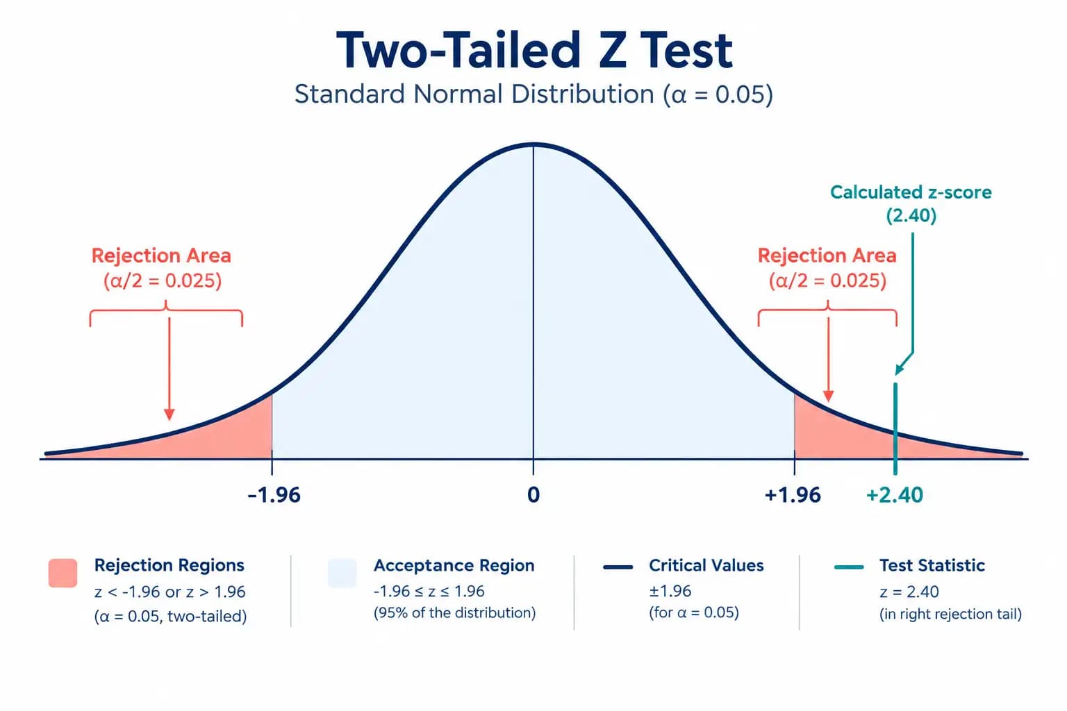
Suppose an industrial bottling facility calibrates machines to dispense 500.0 mL of beverage per bottle. Historical production data confirms that the dispensing process follows a normal distribution with a known population standard deviation () of 4.0 mL.
A quality assurance technician randomly samples 64 bottles from the morning production run. The sample mean () measures 501.2 mL. Does this batch deviate significantly from the 500.0 mL target at a 5% significance level ()?
Step 1: State the Hypotheses
- Null Hypothesis (): (The machine is dispensing correctly).
- Alternative Hypothesis (): (Two-tailed test; the machine is over-dispensing or under-dispensing).
Step 2: Identify the Input Variables
Step 3: Compute the Standard Error of the Mean
Step 4: Calculate the Z Statistic
Step 5: Determine Critical Values and P-Value
For a two-tailed test at , critical boundaries sit at .
The p-value corresponds to the probability of finding .
Using the standard normal distribution table: .
Multiplying by two for both tails gives .
Step 6: Interpret the Result
Because the calculated test statistic () exceeds the upper critical threshold (), and the p-value () is less than our significance level (), we reject the null hypothesis. The quality control engineer has sufficient statistical evidence that the morning bottling line is overfilling bottles, requiring machine recalibration.
How to Interpret Your Z Test Results
Making an informed decision from your test output involves two parallel decision approaches: the Critical Value Approach and the P-Value Approach. Both yield identical conclusions.
The worked example above: z = 2.40 falls in the shaded rejection region beyond ±1.960, so H₀ is rejected.
The P-Value Approach
Compare your calculated p-value directly against your chosen alpha ():
- If : Reject the null hypothesis (). The data provides strong evidence that the observed effect is statistically significant.
- If : Fail to reject the null hypothesis (). The observed difference could easily happen by chance.
The Critical Value Approach
Compare your test statistic () against the critical cutoff values ():
- Two-Tailed Test: Reject if or .
- Left-Tailed Test: Reject if .
- Right-Tailed Test: Reject if .
When planning experimental trials where detecting subtle differences is mandatory, run a sample size calculator beforehand to ensure your study gathers enough observations to achieve adequate statistical power.
Assumptions and Limitations
A z test provides rigorous mathematical guarantees, but only when your dataset satisfies core assumptions:
- Known Population Standard Deviation: The exact population parameter must be known beforehand from historical census data or engineering specifications. If you estimate standard deviation using sample data (), switch to a Student's t-test.
- Normality or Large Sample Size: The underlying population distribution must be normal, or the sample size must be large (). Under the Central Limit Theorem, sampling distributions of the mean approach normality as sample sizes expand.
- Independent Observations: Every measurement must be collected independently. Sampling without replacement from small populations requires finite population corrections.
- Continuous Scale: The measured variable must sit on a continuous ratio or interval scale for mean tests.
Common Mistakes to Avoid
Even seasoned analysts occasionally stumble on subtle statistical nuances:
- Treating Sample Standard Deviation as Population Sigma: Entering sample standard deviation () directly into a z test formula when sample sizes are small () inflates Type I errors. Always use a t-test when population dispersion is unknown.
- Mismatched Tails: Choosing a one-tailed test after seeing the sample mean creates confirmation bias. Specify your alternative hypothesis direction before collecting or examining data.
- Confusing Statistical Significance with Practical Significance: A microscopic difference can become statistically significant () when sample sizes reach tens of thousands. Always inspect raw effect sizes before enacting expensive operational changes.
- Rounding Errors in Intermediate Steps: Rounding the standard error to one decimal place before dividing can shift your computed z-score noticeably. Carry four or more decimal places through intermediate steps.
Frequently Asked Questions
When should I use a z test instead of a t test?
Use a z test when you know the population standard deviation () or when your sample size exceeds 30 with known dispersion. If the population standard deviation is unknown and must be estimated from your sample, use a t-test instead.
Can the z-score be negative?
Yes. A negative z-score simply indicates that your observed sample mean sits below the hypothesized population mean.
What is the difference between a one-tailed and two-tailed z test?
A two-tailed test evaluates whether a sample mean is significantly different in either direction from the null value. A one-tailed test specifically checks for directional differences, testing exclusively whether the mean is greater than or less than the benchmark.
What does a p-value of 0.05 mean?
A p-value of 0.05 means there is a 5% probability of observing a test statistic at least as extreme as the one calculated, assuming the null hypothesis is completely true.
Does a large sample size guarantee valid z test results?
Not necessarily. While large sample sizes fulfill normality requirements via the Central Limit Theorem, they cannot correct for selection bias, measurement flaws, or non-independent sampling methods.
What critical value corresponds to a 95% confidence level?
For a two-tailed test at a 95% confidence level (), the critical z-values are . For a one-tailed test at the same level, the critical value is either or .
Can I run a z test on proportion data?
Yes. The calculator has a one-sample proportion tab and a two-sample proportion tab. The normal approximation to the binomial holds when both and reach 10, which is the threshold the assumption checks apply. Older texts use 5, but 10 is the modern convention and the safer one near the extremes of the proportion scale.
What should I do if my calculated z-score falls exactly on the critical value?
If your test statistic matches the critical value exactly, the p-value equals alpha (). By standard statistical convention, you reject the null hypothesis.